中山大学软件工程数据挖掘第一次作业
线性回归
某班主任为了了解本班同学的数学和其他科目考试成绩间关系,在某次阶段性测试中,他在全班学生中随机抽取1个容量为5的样本进行分析。该样本中5位同学的数学和其他科目成绩对应如下表: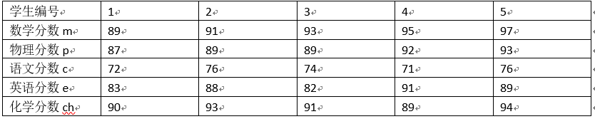
利用以上数据,建立m与其他变量的多元线性回归方程。
梯度下降法代码如下:
1 | import numpy as np |
运行结果如下:
标准方程代码如下:
1 | import numpy as np |
运行结果如下:
正则化的标准方程代码如下:
1 | import numpy as np |
运行结果如下:
scikit-learn线性回归代码如下:
1 | import numpy as np |
运行结果如下: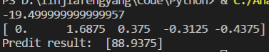
逻辑回归
研究人员对使用雌激素与子宫内膜癌发病间的关系进行了1:1配对的病例对照研究。病例与对照按年龄相近、婚姻状况相同、生活的社区相同进行了配对。收集了年龄、雌激素药使用、胆囊病史、高血压和非雌激素药使用的数据。变量定义及具体数据如下:
match:配比组
case:case=1病例;case=0对照(未发病)
est:est=1使用过雌激素;est=0未使用雌激素;
gall:gall=1有胆囊病史;gall=0无胆囊病史;
hyper:hyper=1有高血压;hyper=0无高血压;
nonest:nonest=1使用过非雌激素;nonest=0未使用过非雌激素;
表格略,表格的数据已在代码中体现。
简单逻辑回归代码如下:
1 | import math |
运行结果如下: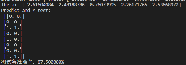
正则化代价函数的逻辑回归代码如下:
1 | import math |
运行结果如下:
scikit-learn逻辑回归代码如下:
1 | from sklearn.linear_model import LogisticRegression |
运行结果如下: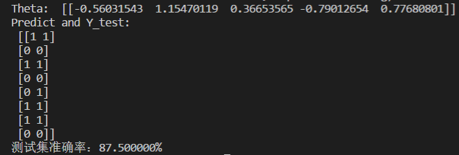
支持向量机
考虑以下的两类训练样本集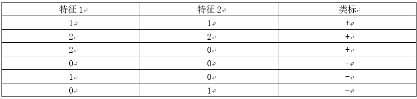
scikit-learn支持向量机代码如下:
1 | import numpy as np |
运行结果如下: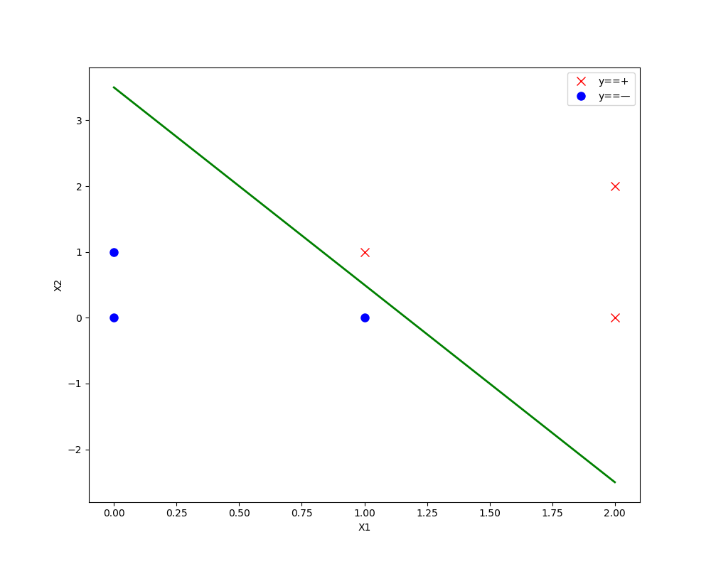
决策边界如下图: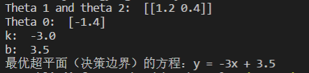
拉格朗日待定乘数求解代码如下:
SMO算法来自这个博客https://blog.csdn.net/willbkimps/article/details/54697698
1 | import numpy as np |
运行结果如下: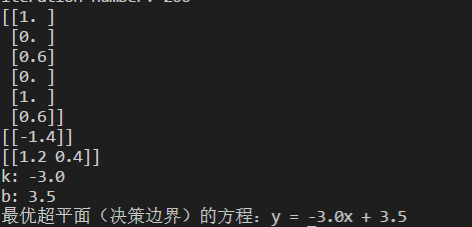
matlab版本的SMO算法:参考这位真大佬https://blog.csdn.net/on2way/article/details/47730367
虽然代码有点小纰漏,我已经在我自己的代码改过来了:
1 | %% |
运行结果如下: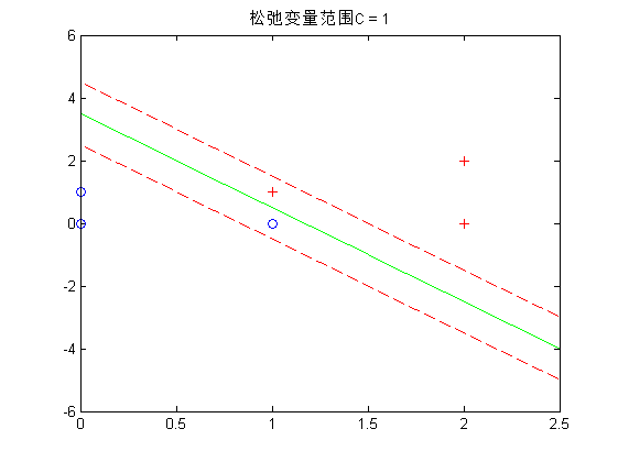
决策边界(绿色线)以及支持向量(红色线)如下: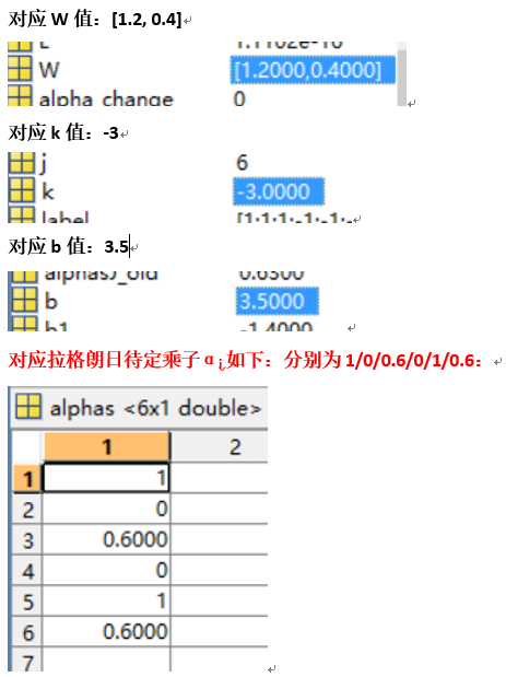
作业思考
- 线性回归与逻辑回归的区别:
线性回归主要用来解决连续值预测的问题,逻辑回归用来解决分类的问题,输出的属于某个类别的概率。 - 逻辑回归与支持向量机的区别:
两种方法都是常见的分类算法,两者的根本目的都是一样的。
目标函数:逻辑回归采用的是logistical loss,svm采用的是hinge loss。这两个损失函数的目的都是增加对分类影响较大的数据点的权重,减少与分类关系较小的数据点的权重。
训练样本点:SVM的处理方法是只考虑support vectors,也就是和分类最相关的少数点,去学习分类器。而逻辑回归通过非线性映射,大大减小了离分类平面较远的点的权重,相对提升了与分类最相关的数据点的权重。
简单性:逻辑回归相对来说模型更简单,容易实现,特别是大规模线性分类时比较方便。而SVM的理解和优化相对来说复杂一些。但是SVM的理论基础更加牢固,有一套结构化风险最小化的理论基础,虽然一般使用的人不太会去关注。还有很重要的一点,SVM转化为对偶问题后,分类只需要计算与少数几个支持向量的距离,这个在进行复杂核函数计算时优势很明显,能够大大简化模型和计算量。